What is Phase Equilibrium?

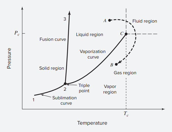
Equilibrium is a condition in which no changes occur in the macroscopic properties of an isolated system with time. At equilibrium, all potentials that may cause change are exactly balanced, so no driving force exists for any change in the system. An isolated system consisting of liquid and vapor phases in intimate contact eventually reaches a final state wherein no tendency exists for change to occur within the system. The temperature, pressure, and phase compositions reach final values which thereafter remain fixed. The system is in equilibrium. Nevertheless, at the microscopic level, conditions are not static. The molecules comprising a phase at a given instant are not the same molecules that later occupy the same phase. Molecules constantly pass from one phase to the other. However, the average rate of passage of molecules is the same in both directions, and no net interphase transfer of material occurs.

VLE and its Applications

Vapor Liquid Equilibrium (VLE) is a subset of phase equilibrium which solely focus on vapor and liquid phase. This subject has a significant rule in chemical engineering as it is widely used for distillation and extraction processes.

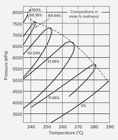
Below, you can see PT diagram of Methanol-Benzyne at equilibrium for several compositions:

What Do We Want From VLE Calculations?

Imagine you have a mixture with a certain composition. Then you have to figure out the distribution of components in the liquid and vapor phase repectively. Or maybe you want to calculate bubble pressure and dew pressure to seprate the components. Nevertheless, VLE calculations, which are consitent of BUBL P and DEW P calculations alongside FLASH calculations, are a vital tool for such analysis.

By completing VLE calculations succesfuly, one can obtain vapor/liquid ratio, vapor phase and liquid phase mole fractions, bubble pressure, dew pressure, fugasity coefficients, Z factors, etc.

Different Models for VLE Calculations

There are several models and equations for VLE calculations intrduced by different sources. The major differences between these models are their precision and complexity. Here a number of famous and widely used models are briefly introduced:

1. Raoult's Law

In this model, it is assumed that both the vapor and liquid mixtures are ideal. These assumptions are acceptable in low pressures but in higher pressures, this model shows great derivation from experimaental data. The formulation of this model is as follows:

$$y_i P=x_i P_i^{sat}$$
2. Henry's Law

In a case where the tempreture of the system is higher than the critical temperature of a component, Raoult's Law can not be applied because Antoine Equations can not be used for saturated pressure calculations anymore. Thus, a new parameter is introduced as below:

$$y_i P=x_i H_i$$

where H values must be obtained experimentaly.

3. Modified Raoult's Law

As evident from the name, this model is an enhaned version of the original Raoult's Law. This is achieved by entering a new variable called activity coefficient into the equation:

$$y_i P=x_i \gamma_i P_i^{sat}$$

This new parameter is either determined by experiment or using comlicated models that are built uppon experimental data.

4. Gamma/Phi Formulation

This model is an advanced and relatively accurate model for VLE calculations where takes into account both the non-ideality of vapor and liquid phases by utilizing fugasity coefficients and activity coefficients:

$$y_i \Phi_i P=x_i \gamma_i P_i^{sat}$$

where:

$$\Phi_i = \frac{\Phi_i^v}{\Phi_i^{sat}} exp \frac{-V_i^l(P-P_i^{sat})}{RT}$$

Major problems with this model is the calculation of activity coefficient and the fact that it still uses saturated pressure which is not defined for temperatures above critical tempreture of the component.

5. Phi/Phi Model

The best way to calculate VLE problems with minimum data required and best accuracy is Phi/Phi model which will be discussed in the next section.

Why Phi/Phi model?

Phi/Phi model is where accuracy and simplicity meet each other. It requires a small number of parameters and is done by utilizing Equation of State models to calculate fugacity coefficients which can be further used to calculate the desired parameters like mole fractions of each phase.

The main concept in phase equilibrium is that the fugacity of each component is the same for all phases:

$$\hat{f}_i^v = \hat{f}_i^l$$

By definition, an alternative form for the equation above is:

$$y_i P \hat{\Phi}_i^v = x_i P \hat{\Phi}_i^l$$

which can be reduced to:

$$y_i \hat{\Phi}_i^v = x_i \hat{\Phi}_i^l$$

As you can see, this model only requiers fugacity coefficient, which can be obtained from EoS and will be discussed later.

Phi/Phi Model calculation Flow Chart

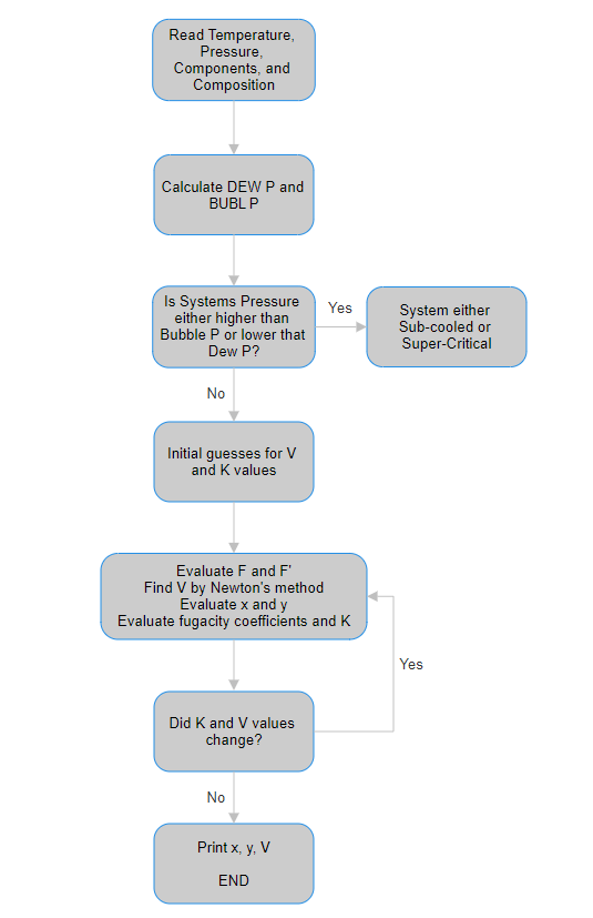
All the necessary formulas and parameters will be defined in the next sections.

F, F', and V Calculation

As shown in the flow chart above, F, F', and V values are required to be calculated. But first of all, an initial guess for V value in required which is done as below:

$$V = \frac{P_{bubl} - P}{P_{bubl} - P_{dew}}$$

Moreover, F and F' can be evaluated as below:

$$F = \sum_i \frac{z_i (K_i - 1)}{1+V(K_i-1)}$$ $${F'} = \frac{\text{d}F}{\text{d}V} =- \sum_i \frac{z_i (K_i - 1)^2}{[1+V(K_i-1)]^2}$$

When F, F', K, and V is determined, mole fractions of both phases can be evaluated:

$$x_i = \frac{z_i}{1+V(K_i-1)}$$ $$y_i = x_i K_i$$

BUBL P & DEW P Calculation

Bubble Pressure and Dew Pessure calcualtions are very common in chemical engineering calculations and are widely used in several related fields like distillation, seperation, thermodynamic behavior simulation, etc.

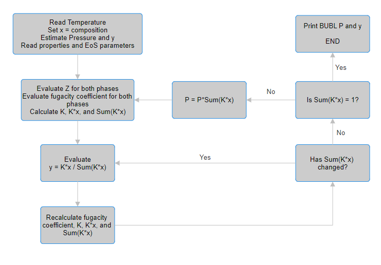
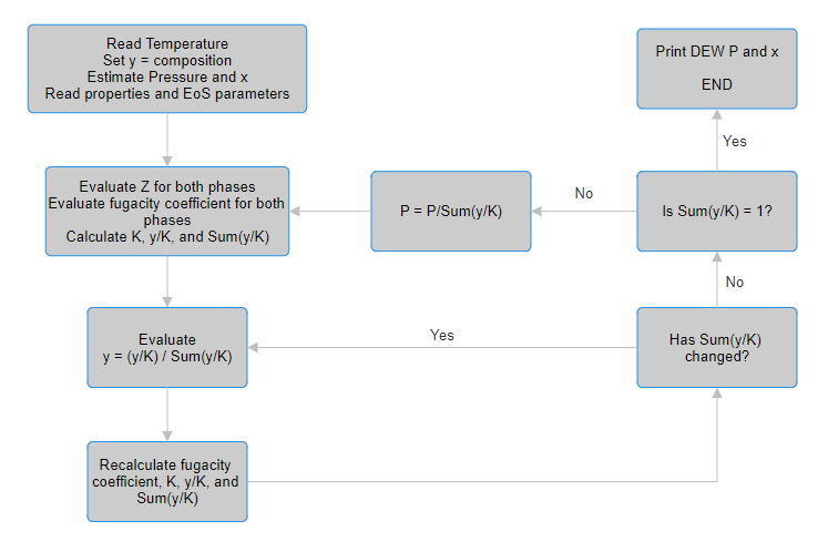
In the Phi/Phi formulation, fugacity coefficients are used to evaluate K values and then iterate for pressure value while chekcing the mole fractions and pressures to see if bubble/dew point has been reach or not.

$$K_i = \frac{y_i}{x_i} = \frac{\hat{\Phi}_i^l}{\hat{\Phi}_i^v}$$

In the next two sections, flow charts for BUBL P and DEW P calculations are provided.

Initial values for P and K is required for the first iteration. This can be achieved by the following correlations:

$$ln P_r^{initial} = f^{(0)} + \omega f^{(1)}$$

where

$$P_r = \frac{P}{P_c}$$ $$f^{(0)} = 5.92714 - \frac{6.09648}{T_r} - 1.28862 \ln{T_r} + 0.169347 \ln{T_r^6}$$ $$f^{(1)} = 15.2518 - \frac{15.6875}{T_r} - 13.4721 \ln{T_r} + 0.43577 \ln{T_r^6}$$

and K can be estimated as below:

$$K_i^{initial} = \frac{1}{P_{r,i}} \exp{5.37 (1+\omega_i)(1 - \frac{1}{T_{r,i}})}$$

BUBL P Calculation Flow Chart

DEW P Calculation Flow Chart

Equations of State (EoS)

Compressibility Factor (Z) is a parameter which accounts for the non-ideality of a mixture or system:

$$Z = \frac{PV}{RT}$$

Z factor is in our interests because its value is required for calculation of fugacity factor, which is the main parameter in VLE calculations. There are several models and formulation of EoS that each have their own pros and cons. Here are a few famous ones:

• van der Waals (vdW)
• Redlich - Kwong (RK)
• Soave - Redlich - Kwong (SRK)
• Peng - Robinson (PR)

Among the models above, the Peng-Robinson model leads to better results in an overall point of view. Thus, this model is be used in further modellings and calculations.

After choosing the desired EoS model, parameters and constants must be evaluated. Next, roots of the cubic equation must be found in order to determine the vapor phase and liquid phase Z factor. A thorough and complete documentation about Peng-Robinson EoS parameters and a easy-to-follow guide on Solution Techniques for Cubic Expressions & Root Finding is provided that are highly recommended and are used in this project extensively.

Fugacity Coefficient

As mentioned before, the main parameter in Phi-Phi model for VLE calculations is the Fugacity Coefficient. After calculating the Z factor and evaluating the required parameters related to the compessibility factor, fugacity coefficient can be evaluated with ease. For a deeper understanding of the calculation methods used for fugacity coefficient you can check this link.

Required Properties

PEC has the advantage of using such models that require just a few parameters and properties and the main job is done through iteration and models that are precisely developed for such calculations. The only parameters required for such calculations are Critical Temperature, Critical Pressure, Acentric Coefficient, and EoS Parameters.

References

• Solution Algorithms for VLE Problems
• Cubic EOS Fugacity Expressions
• PT Flash Calculation using PR EOS
• Lee - Kesler method
• Intoduction to Chemical Engineering Thermodynamics